Crete Partitioned Table by SQL Server Management Studio and T-SQL script

This blog is about Create Partitioned Tables via T-SQL script and SQL Server Management Studio. Partitioning can make large tables and indexed more manageable and scalable. The data in partition tables and indexed is horizontally divided into units that can be spread across more than one file group in a database. SQL Server 2012 supports up to 15,000 partitions by default. In earlier versions, the number of partitions was limited to 1,000 by default. On x86-based systems, creating a table or index with more than 1000 partitions is possible, but is not supported.

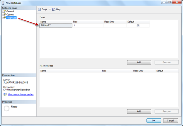
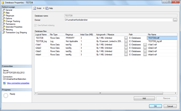
Once you create a new database, you can see there is default file group called PRIMARY as shown below.

The following steps are needed to follow to create a partition via SQL Server Management Studio.

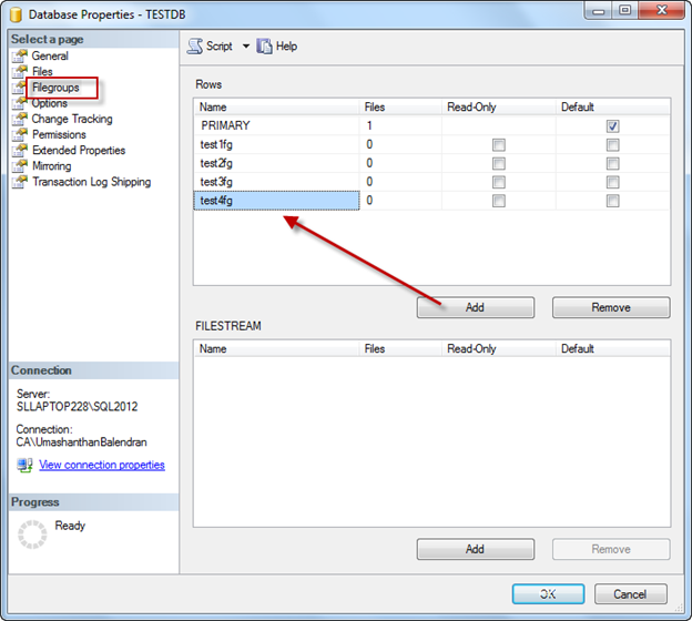
Step 1: Add 4 more file group

Step 2: Add 4 files and assign to each file group.

Step 3: To create partition use Create partition wizard, by right click on particular table

Step 4: Select the column in a table to apply for partition.

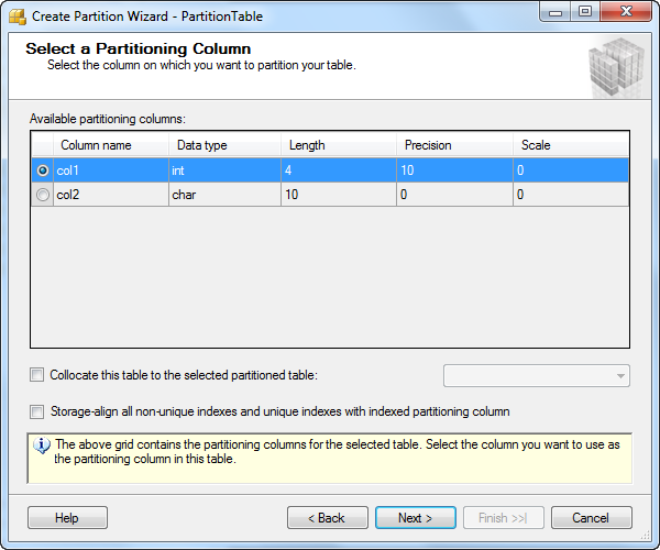
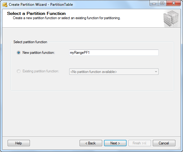
Step 5: Type the Partition Function name

Step 6: Type Partition Scheme name

Step 7: Define the boundary for each file group

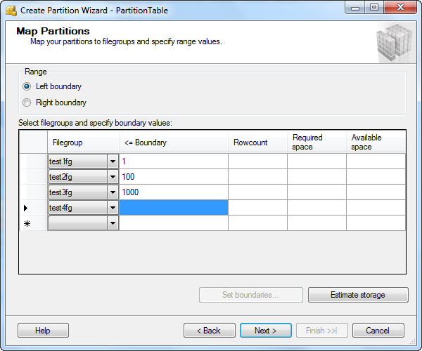
Step 8: You can create the script for these and run it alter or run immediately.

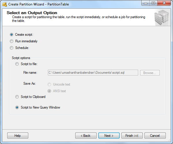
Step 9: insert some values and check whether values are inserting into appropriate file group.

In the same way the following steps have to follow for create partition using T-SQL script.

Create 4 new measure group called test1fg, test2fg, test3fg and test4fg.

Once you run this script you will see there will be 4 more measure group will be available in the database. After that create file group, you have to a create file and add to each file group, for the best practice each file in a different drive would increase the performance.

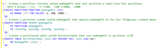
You need to create Partition Function, Partition Scheme and then assign this partition function to the relevant table. In here I have created Partition Function called myRangePF1 using integer value with 3 parameters; in this case there will be 4 ranges

1.       <=1

2.       >1 and <=100

3.       >100 and <=1000

4.       >100

On the Map Partitions page, under Range, select either Left boundary or Right boundary to specify whether to include the highest or lowest bounding value within each filegroup you create. You must always enter one extra filegroup in addition to the number of filegroups specified for the boundary values when you are creating partitions.

In here I created sample table called Partition Table with two column one is integer and another one character field and then assign integer column into Partition Function. The below screen shot will make you clear.

When I insert -1, you will be see that it will insert into test1fg file group as shwon below.

Cheers!

How to create Environmental Variable for Package Configuration in SSIS 2012 (Package Deployment Model) and SSIS 2008

First you need to create Environment al variable, by right click on my computer and properties. Under Advanced tab, click on Environmental variables button, under system variables create a variable as you want. The steps are shown by screen shots.

Cheers!

How to skip first few rows when extract data from Excel sheet

How to read data from Excel nth Row

Most of you might face this common problem that records are not in the common format in excel sheet reports as column header is on first row and records are following. Here I am try to explain one of the real scenario which I had faced.

In this below excel sheet, you can see that records are beginning from 6th row(B6) and 2nd column(B).

  

There so many ways to handle this, for me the easiest way is to use SQL Command in Excel Source as show below.

The Excel Connection Manager is not supported in the 64-bit version of SSIS

If you find the error message as shown below while import data from Excel files, to resolve this issue make it Run64BitRuntime as FALSE under project properties.

[Connection manager "Excel Connection Manager"] Error: SSIS Error Code DTS_E_OLEDB_EXCEL_NOT_SUPPORTED: The Excel Connection Manager is not supported in the 64-bit version of SSIS, as no OLE DB provider is available.

What is MDX, DMX and XMLA - SSAS Languages

These are just definitions and very basic information. You might see that there are 3 kind of language available to work on SSAS via SQL Server Management Studio. They are DMX, MDX and XMLA.

MDX: Multidimensional Expressions, this language is useful to retrieve data from SSAS objects same as T-SQL or SQL in Relational Databases.

DMX: Data Mining Extensions, this language is used for SSAS object, but especially for data mining structure. DMX statements are used to create process, delete, copy, browse, and predict against data mining models.

XMLA: XML for Analysis is a Simple Object Access protocol (SOAP) - based XML protocol, designed specifically for universal data access to any standard multidimensional data source residing on the Web. Microsoft SQL Server Analysis Services implements XMLA per the XMLA 1.1 specification. XMLA is the native protocol for SSAS, used for all interaction between a client application and instance of Analysis Service. Both Analysis Management Objects (AMO) and ADOMD.NET use the XMLA protocol when communicating with an instance of Analysis Service. This XMLA Queries are mainly used for Administrative purposes such as taking backup, moving data, etc.

Cheers!

Database diagram support objects cannot be installed because this database does not have a valid owner

When I try to create a new Diagram the following error message is pop up in SQL Server 2012:

Database diagram support objects cannot be installed because this database does not have a valid owner.  To continue, first use the Files page of the Database Properties dialog box or the ALTER AUTHORIZATION statement to set the database owner to a valid login, then add the database diagram support objects.

Solution: After running this command this problem was solved. Here TESTDW is a database name.

How to create Fact Dimension or Degenerate Dimension

Sometimes additional data in fact table might useful for users such as invoice number, purchase order numbers, some text fields like comments and complaints. When we define dimension based on a fact table item, the dimension is called a fact dimension and also known as degenerate dimension. The reason that we keep the data in fact table instead of having in separate dimension table is the dimension table would grow at the same rate as the fact table, and would just create duplicate data and unnecessary complexity.

For example: In adventure work data base FactInternetSales table has Sales Order Number. User might need to get the sales amount based on SalesOrderNumber.

Let see how to create Fact Dimension for this scenario. Create new dimension.

In Main table select InternetSales, and under key columns add “SalesOrderNumber” and “SalesOrderLineNumber”, under Name column Select SalesOrderLineNumber.

Unchecked all the Related tables

Select Sales Order Number, if you need some more details such as Customer PO Number.

One you create dimension, rename the attribute name as you want. Here I renamed Sales order Number as Item Details, and under name column select the EnglishProductName from product table.

Add the salesOrderNumber again into attribute panel, and set the name as Order Number and Order by Key.

You can choose the storage mode based on the requirement.

Add this new dimension in the cube .

Make sure that this dimension and the Measure Group relationship type as Fact under Dimension usage.

Now you can test the dimension as below.

Cheers!

You might see that parent level member duplicate under leaf level, for this there is a property called “MemberWithData” set as “NonLeafDataHidden” for parent member. By default it set as "NonLeafDataVissible".

Cheers!

Measure Aggregate Functions - SSAS 2012

In SQL Server Analysis Services Enterprise Edition, there are many Aggregate Functions

are available as shown below. In this blog I am going to explain one by one. All the aggregate functions are available only in SSAS Enterprise edition, for example “None” is only available in Enterprise Edition if you try to use in standard edition it will throw an error.

When you create new measure, first thing is you need to select the Aggregation Function that shows as Usage.

Sum: Calculates the sum of values for all child members. This is the default aggregation function.

Count: Retrieves the count of all the child members.

 

Min: Retrieves the lowest value for all child members.

Max: Retrieves the highest value for all child members.

Distinct Count: Retrieves the count of all child members. A few of the more typical application for DISTINCT COUNT analysis are:

• Sales and Marketing, especially counting distinct number of customers.
• Insurance claims relating policies to damages. One claim may have many damages.
• Quality control data relating causes to defects. A defect can be caused by multiple factors.

The below example shows that how distinct count is different from other aggregation functions.

Product Dimension Members	Distinct Customers Count
All products	200
Hardware	80
Computers	70
Monitors	60
Printers	30
Software	150
Home	100
Business	100
Games	80

In this example, 70 customers bought computers, 30 customers bought printers, and 60 customers bought monitors. However, the total number of customers who bought hardware, according to the result set, is not 160, or 70+60+30, as shown in the table. The query results display an actual count of 80 total hardware customers. The reason for this irregularity is simple: many customers bought more than one product. Some customers bought both computers and monitors, others bought the whole three-piece package, and some replaced just the monitor, and so on. The end result is that there is no way to infer directly from the lower level results what the customer subtotal really is. This discrepancy continues through the upper levels as well: 80 customers bought hardware, 150 bought software, and all together, All Products totals only 200 customers.

None:  No aggregation is performed, and all values for leaf and nonleaf members in a dimension are supplied directly from the fact table for the measure group .if no value can be read from the fact table for a member, the value for that member is set to null.

By Account: calculates the aggregation according to the aggregation function assigned to the account type for a member in an account dimension. If no account type dimension exists in the measure group, treated as the Non aggregation functions.

Account type can be defined by unary operations as below:

In here ~ operator meaning ignore aggregation and + operator meaning add to preceding sibling likewise aggregation will be based on particular column value. As this brought subject, I will cover these details of this on other blog.

Average of Children: (Average over time) this is only along a Time Dimension.

Example creates a measure using the sum aggregation type for Sales Amount; create a Non-Empty value or (count of Row) measure as Count, from these we can calculate a measure as

[Measures].[Sales Amount]/[Measures].[Count].

Another important consideration, which depends on the business scenario, is the type of the Count aggregate. It could be Count of rows (Row Bound) or Count of non-empty values. The difference is whether we want to include or exclude the empty values from our aggregate. Either way, the described technique will work equally well.

FirstChild: Retrieves the value of the first child member.

LastChild: Retrieves the values of the last child member.

FirstNonEmpty : Retrieves the value of the first non-empty child member.

 

LastNoneEpty:  Retrieves the value of the last non-empty child member.

Cheers!

By Default, a year level was expected. No such level was found in the cube

When you use YTD function in KPI or calculated measures, you might get the error message as “By Default, a year level was expected. No such level was found in the cube”. The reason for this is most of the date dimensions are formed based on pre populated Date Dimension table, so the SSAS Engine itself not able to find the Field which is Year.

The solution for this, have to manually define which Filed is Year filed in Date Dimension table. Simply you can use Business Intelligence Wizard to define the Year filed as shown below.

If not we can define using the field properties “Type” set as relevant Type. The below image shows that a field in the date dimension is been set as Quarter Type.

Cheers!